Advanced tutorial for query to reference mapping using expiMap with de novo learned gene programs

[1]:

import warnings
warnings.simplefilter(action='ignore')

[2]:

import scanpy as sc
import torch
import scarches as sca
import numpy as np
import gdown

Global seed set to 0

[3]:

sc.set_figure_params(frameon=False)
sc.set_figure_params(dpi=200)
sc.set_figure_params(figsize=(4, 4))
torch.set_printoptions(precision=3, sci_mode=False, edgeitems=7)

Download reference and do preprocessing

[4]:

url = 'https://drive.google.com/uc?id=1Rnm-XKEqPLdOq3lpa3ka2aV4bOXVCLP0'
output = 'pbmc_tutorial.h5ad'
gdown.download(url, output, quiet=False)

Downloading...
From: https://drive.google.com/uc?id=1Rnm-XKEqPLdOq3lpa3ka2aV4bOXVCLP0
To: C:\Users\sergei.rybakov\projects\notebooks\pbmc_tutorial.h5ad
100%|███████████████████████████████████████████████████████████████████████████████| 231M/231M [00:42<00:00, 5.39MB/s]

[4]:

'pbmc_tutorial.h5ad'

[4]:

adata = sc.read('pbmc_tutorial.h5ad')

.X should contain raw counts.

[5]:

adata.X = adata.layers["counts"].copy()

Read the Reactome annotations, make a binary matrix where rows represent gene symbols and columns represent the terms, and add the annotations matrix to the reference dataset. The binary matrix of annotations is stored in adata.varm['I']. Note that only terms with minimum of 12 genes in the reference dataset are retained.

[ ]:

url = 'https://drive.google.com/uc?id=1136LntaVr92G1MphGeMVcmpE0AqcqM6c'
output = 'reactome.gmt'
gdown.download(url, output, quiet=False)

[6]:

sca.utils.add_annotations(adata, 'reactome.gmt', min_genes=12, clean=True)

Remove all genes which are not present in the Reactome annotations.

[7]:

adata._inplace_subset_var(adata.varm['I'].sum(1)>0)

For a better model performance it is necessary to select HVGs. We are doing this by applying the scanpy.pp function highly_variable_genes(). The n_top_genes is set to 2000 here. However, for more complicated datasets you might have to increase number of genes to capture more diversity in the data.

[8]:

sc.pp.normalize_total(adata)

[9]:

sc.pp.log1p(adata)

[10]:

sc.pp.highly_variable_genes(
    adata,
    n_top_genes=2000,
    batch_key="batch",
    subset=True)

Filter out any annotations (terms) with less than 12 genes.

[11]:

select_terms = adata.varm['I'].sum(0)>12

[12]:

adata.uns['terms'] = np.array(adata.uns['terms'])[select_terms].tolist()

[13]:

adata.varm['I'] = adata.varm['I'][:, select_terms]

Filter out genes not present in any retained terms after selection of HVGs.

[14]:

adata._inplace_subset_var(adata.varm['I'].sum(1)>0)

Put the count data back to adata.X.

[15]:

adata.X = adata.layers["counts"].copy()

Example with constrained and unconstrained extension nodes

Later, we will use a query dataset that contains IFN-beta stimulated and unstimulated PBMC cells.

Here, we remove some Interferon beta and B cell specific signals from the reference by dropping some related terms from the annotation matrix. The signals corresponding to these terms will be recovered later with the extension nodes added in the query at the surgery step.

Select the interferon beta annotations from the loaded Reactome pathway database for removal.

[16]:

rm_terms = ['INTERFERON_SIGNALING', 'INTERFERON_ALPHA_BETA_SIGNALIN',
            'CYTOKINE_SIGNALING_IN_IMMUNE_S', 'ANTIVIRAL_MECHANISM_BY_IFN_STI']

Select the annotations related to B cells for removal.

[17]:

rm_terms += ['SIGNALING_BY_THE_B_CELL_RECEPT', 'MHC_CLASS_II_ANTIGEN_PRESENTAT']

[18]:

ix_f = []
for t in rm_terms:
    ix_f.append(adata.uns['terms'].index(t))

Store the ‘SIGNALING_BY_THE_B_CELL_RECEPT’ annotation separately.

[19]:

query_mask = adata.varm['I'][:, ix_f[4]][:, None].copy()

Remove the selected annotations.

[20]:

adata.varm['I'] = np.delete(adata.varm['I'], ix_f, axis=1)

[21]:

adata.uns['terms'] = [term for term in adata.uns['terms'] if term not in rm_terms]

Remove B cells from the reference.

[22]:

rm_b = ["B", "CD10+ B cells"]

[23]:

adata = adata[~adata.obs['cell_type'].isin(rm_b)].copy()

Train the reference.

[24]:

intr_cvae = sca.models.EXPIMAP(
    adata=adata,
    condition_key='study',
    hidden_layer_sizes=[300, 300, 300],
    recon_loss='nb'
)


INITIALIZING NEW NETWORK..............
Encoder Architecture:
        Input Layer in, out and cond: 1972 300 4
        Hidden Layer 1 in/out: 300 300
        Hidden Layer 2 in/out: 300 300
        Mean/Var Layer in/out: 300 276
Decoder Architecture:
        Masked linear layer in, ext_m, ext, cond, out:  276 0 0 4 1972
        with hard mask.
Last Decoder layer: softmax

See https://docs.scarches.org/en/latest/training_tips.html for the recommendation on hyperparameter choice.

[25]:

ALPHA = 0.7

[26]:

early_stopping_kwargs = {
    "early_stopping_metric": "val_unweighted_loss",
    "threshold": 0,
    "patience": 50,
    "reduce_lr": True,
    "lr_patience": 13,
    "lr_factor": 0.1,
}
intr_cvae.train(
    n_epochs=400,
    alpha_epoch_anneal=100,
    alpha=ALPHA,
    alpha_kl=0.5,
    weight_decay=0.,
    early_stopping_kwargs=early_stopping_kwargs,
    use_early_stopping=True,
    seed=2020
)

Init the group lasso proximal operator for the main terms.
 |██████████████------| 72.2%  - val_loss: 935.2109799592 - val_recon_loss: 909.6967879586 - val_kl_loss: 51.0283828404208
ADJUSTED LR
 |███████████████-----| 76.8%  - val_loss: 934.3165150518 - val_recon_loss: 908.9699786642 - val_kl_loss: 50.6930810680
ADJUSTED LR
 |████████████████----| 80.2%  - val_loss: 934.5560806938 - val_recon_loss: 909.1601987092 - val_kl_loss: 50.7917618130
ADJUSTED LR
 |████████████████----| 83.5%  - val_loss: 934.7631597104 - val_recon_loss: 909.4011548913 - val_kl_loss: 50.7240132871
ADJUSTED LR
 |█████████████████---| 86.8%  - val_loss: 934.5707238239 - val_recon_loss: 909.2114868164 - val_kl_loss: 50.7184793224
ADJUSTED LR
 |█████████████████---| 89.5%  - val_loss: 934.3915139903 - val_recon_loss: 909.0323433254 - val_kl_loss: 50.7183265686
Stopping early: no improvement of more than 0 nats in 50 epochs
If the early stopping criterion is too strong, please instantiate it with different parameters in the train method.
Saving best state of network...
Best State was in Epoch 306

Referece mapping while learning new varation from query data with extension nodes

The Kang dataset contains control and IFN-beta stimulated cells. We use this as the query dataset.

[ ]:

url = 'https://drive.google.com/uc?id=1t3oMuUfueUz_caLm5jmaEYjBxVNSsfxG'
output = 'kang_tutorial.h5ad'
gdown.download(url, output, quiet=False)

[27]:

kang = sc.read('kang_tutorial.h5ad')[:, adata.var_names].copy()

[28]:

kang.obs['study'] = 'Kang'

[29]:

kang.uns['terms'] = adata.uns['terms']

Add 3 unconstrained (to capture de novo programs) and one constrained nodes, where the constrain represents the ‘SIGNALING_BY_THE_B_CELL_RECEPT’ term. Note that this term was dropped when the reference model was learned. Also use HSIC regularization for the unconstrained nodes to encourge independence of learned de novo gene programs.

[30]:

q_intr_cvae = sca.models.EXPIMAP.load_query_data(kang, intr_cvae,
                                                 unfreeze_ext=True,
                                                 new_n_ext=3,
                                                 new_n_ext_m=1,
                                                 new_ext_mask=query_mask.T,
                                                 new_soft_ext_mask=True,
                                                 use_hsic=True,
                                                 hsic_one_vs_all=True
                                                )


INITIALIZING NEW NETWORK..............
Encoder Architecture:
        Input Layer in, out and cond: 1972 300 5
        Hidden Layer 1 in/out: 300 300
        Hidden Layer 2 in/out: 300 300
        Mean/Var Layer in/out: 300 276
        Expanded Mean/Var Layer in/out: 300 4
Decoder Architecture:
        Masked linear layer in, ext_m, ext, cond, out:  276 1 3 5 1972
        with hard mask.
Last Decoder layer: softmax

Train with hypeparameters:

gamma_ext - L1 regularization coefficient for the new unconstrained nodes. Specifies the strength of sparcity enforcement for these nodes.

gamma_epoch_anneal - number of epochs for gamma_ext annealing.

alpha_l1 - L1 regularization coefficient for the soft mask of the new constrained node.

beta - HSIC regularization coefficient for the unconstrained nodes, enforces their independence from the old reference nodes and from each other if hsic_one_vs_all=True.

[31]:

q_intr_cvae.train(
    n_epochs=250,
    alpha_epoch_anneal=120,
    alpha_kl=0.22,
    weight_decay=0.,
    alpha_l1=0.96,
    gamma_ext=0.7,
    gamma_epoch_anneal=50,
    beta=3.,
    seed=2020,
    use_early_stopping=False
)

Init the L1 proximal operator for the unannotated extension.
Init the soft mask proximal operator for the annotated extension.
 |████████████████████| 100.0%  - val_hsic_loss: 0.2133808624 - val_loss: 517.5771179199 - val_recon_loss: 501.4962740811 - val_kl_loss: 70.1850114302

Analysis of the extension nodes for reference + query dataset

[32]:

kang_pbmc = sc.AnnData.concatenate(adata, kang, batch_key='batch_join', uns_merge='same')

[33]:

kang_pbmc.obs['condition_joint'] = kang_pbmc.obs.condition.astype(str)
kang_pbmc.obs['condition_joint'][kang_pbmc.obs['condition_joint'].astype(str)=='nan']='control'

This adds extension nodes’ names to kang_pbmc.uns['terms'].

[34]:

q_intr_cvae.update_terms(adata=kang_pbmc)

[35]:

q_intr_cvae.latent_directions(adata=kang_pbmc)

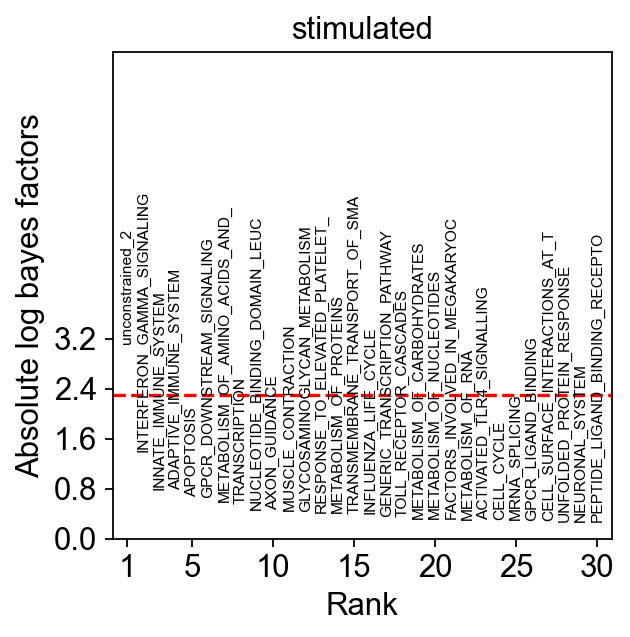
Do gene set enrichment test for condition in reference + query using Bayes Factors.

[36]:

q_intr_cvae.latent_enrich(groups='condition_joint', comparison='control', use_directions=True, adata=kang_pbmc)

[37]:

fig = sca.plotting.plot_abs_bfs(kang_pbmc, yt_step=0.8, scale_y=2.5, fontsize=7)

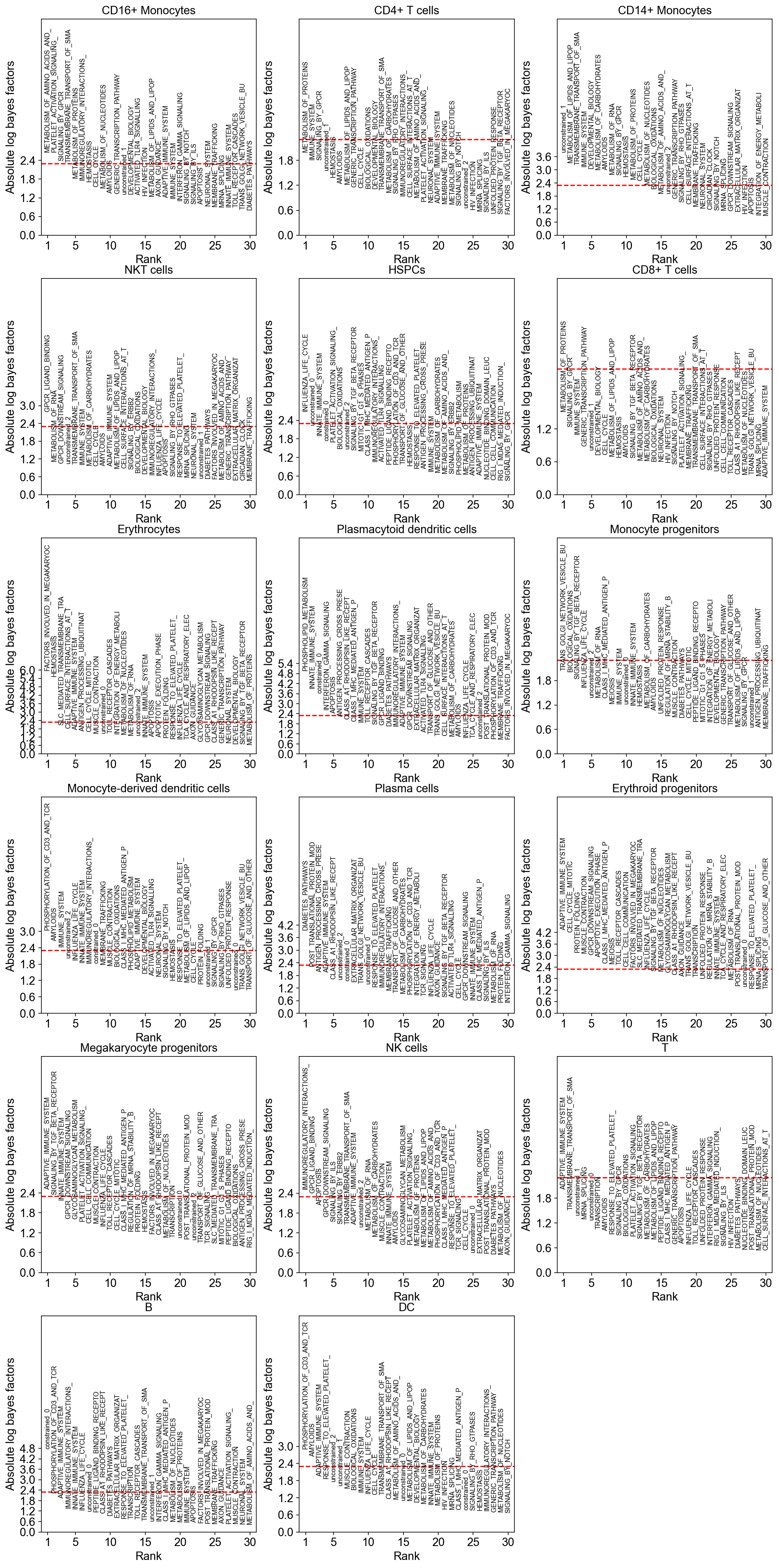
_images/expimap_surgery_pipeline_advanced_64_0.png

Do gene set enrichment test for cell types in reference + query control using Bayes Factors.

[38]:

kang_pbmc_control = kang_pbmc[kang_pbmc.obs['condition_joint']=='control'].copy()

q_intr_cvae.latent_enrich(groups='cell_type', use_directions=True, adata=kang_pbmc_control, n_sample=10000)

[ ]:

fig = sca.plotting.plot_abs_bfs(kang_pbmc_control, n_cols=3, scale_y=2.6, yt_step=0.6)

[40]:

fig.set_size_inches(16, 34)

[41]:

fig

[41]:

_images/expimap_surgery_pipeline_advanced_69_0.png

Plot the latent variables for query + reference corresponding to the constrained and unconstrained extension nodes.

[42]:

terms = kang_pbmc.uns['terms']
select_terms = ['constrained_0', 'unconstrained_0', 'unconstrained_1', 'unconstrained_2']
idx = [terms.index(term) for term in select_terms]

[43]:

latents = (q_intr_cvae.get_latent(kang_pbmc.X, kang_pbmc.obs['study'], mean=False) * kang_pbmc.uns['directions'])[:, idx]

[44]:

kang_pbmc.obs['constrained_0'] = latents[:, 0]

kang_pbmc.obs['unconstrained_0'] = latents[:, 1]
kang_pbmc.obs['unconstrained_1'] = latents[:, 2]
kang_pbmc.obs['unconstrained_2'] = latents[:, 3]

[45]:

sc.pl.scatter(kang_pbmc, x='unconstrained_2', y='constrained_0', color='condition_joint', size=10)

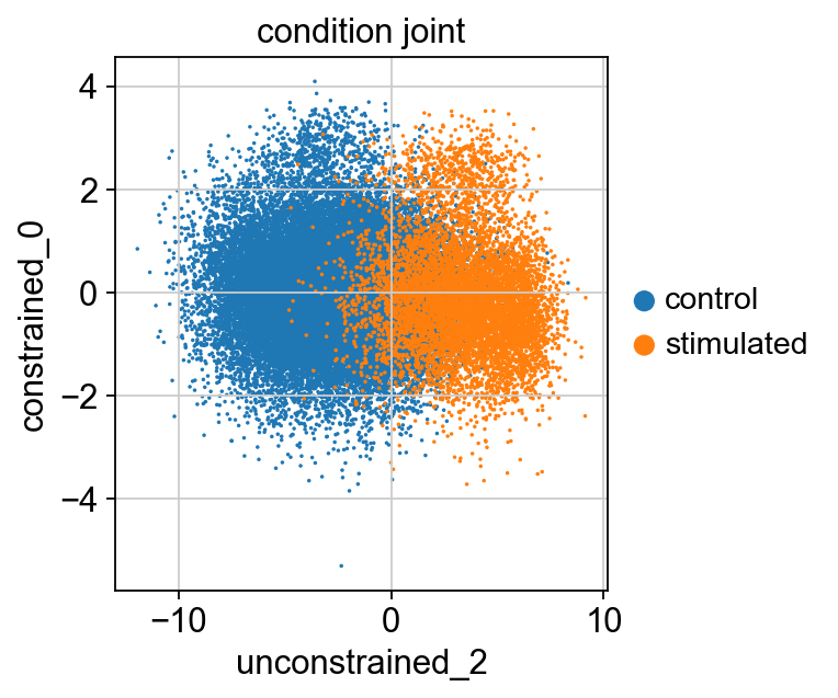
_images/expimap_surgery_pipeline_advanced_74_0.png

Note that the signal associated with the program learned by unconstrained_2 was enriched in stimulated condition compared to control. Here, the cells are separated by their latent scores for unconstrained_2, which suggests that this node is indeed capturing the variation induced by IFN-beta stimulation.

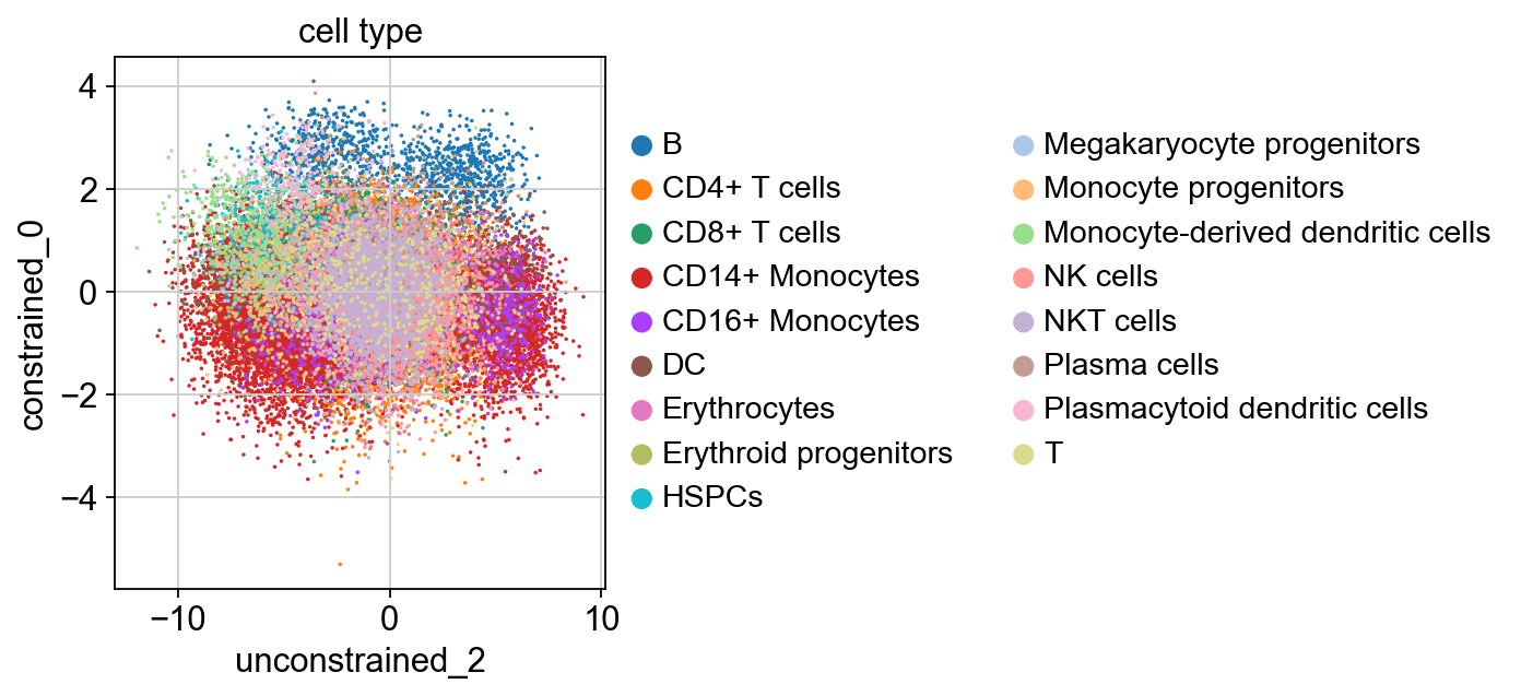
[46]:

sc.pl.scatter(kang_pbmc, x='unconstrained_2', y='constrained_0', color='cell_type', size=10)

_images/expimap_surgery_pipeline_advanced_76_0.png

[47]:

sc.pl.scatter(kang_pbmc, x='unconstrained_1', y='unconstrained_0', color='cell_type', size=10)

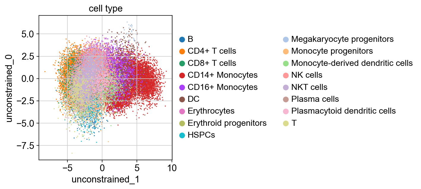
_images/expimap_surgery_pipeline_advanced_77_0.png

Recall that unconstrained_1 was differentially enriched in CD14+ Monocytes. Therefore, this node is capturing the CD14+ Monocyte cell type variation.

Get genes from extension nodes sorted by their absolute weights in the decoder. Higher absolute value of the weight means that this gene is affected more by the gene program.

[48]:

q_intr_cvae.term_genes('constrained_0', terms=kang_pbmc.uns['terms'])

[48]:

	genes	weights	in_mask
0	CD79A	-1.686799	True
1	BLK	-1.411135	True
2	CD19	-1.384097	True
3	BLNK	-1.166159	True
4	CD79B	-1.164143	True
...	...	...	...
66	STIM1	-0.000940	True
67	CERS4	-0.000227	False
68	HLA-DPB1	-0.000045	False
69	HLA-A	0.000036	False
70	KCNG1	-0.000012	False

71 rows × 3 columns

[51]:

q_intr_cvae.term_genes('unconstrained_1', terms=kang_pbmc.uns['terms'])

[51]:

	genes	weights	in_mask
0	RGS2	3.689368e-01	False
1	CCL2	-3.177418e-01	False
2	TIMP1	-3.089722e-01	False
3	PLA2G7	-2.966527e-01	False
4	GMPR	-2.102084e-01	False
...	...	...	...
486	PNPLA8	1.008977e-05	False
487	HS2ST1	8.462230e-06	False
488	SLC25A13	-7.957511e-06	False
489	SLC4A2	-3.113702e-06	False
490	EBF1	3.527966e-07	False

491 rows × 3 columns

[50]:

q_intr_cvae.term_genes('unconstrained_2', terms=kang_pbmc.uns['terms'])

[50]:

	genes	weights	in_mask
0	IFIT3	-0.341521	False
1	IFIT1	-0.338443	False
2	IFIT2	-0.335060	False
3	CXCL10	-0.334820	False
4	ISG15	-0.332265	False
...	...	...	...
391	ZNF235	-0.000018	False
392	ILK	-0.000017	False
393	RGS2	0.000017	False
394	SLC44A1	0.000006	False
395	FURIN	0.000003	False

396 rows × 3 columns

Note that unconstrained_2 was capturing the variation induced by IFN-beta stimulation. Here, the genes from the Interferon Induced Protein gene family have the largest absolute weights in the program captured by this unconstrained node, certifying that the learned program is indeed capturing variations in gene expression due to activity of the inteferon signalling, which was induced by IFN-beta stimulation.